Tutorials

This documentation goes over how to use Smart Curriculum Designer, the machine learning and AI curriculum generator. The application itself enables educators to generate models, content, exercises, and solutions, weaving the domain/dataset specified by the educator.

---

Getting Started

This application uses Tapis, if you already have an account and a system authenticated you may skip this section.

1. Navigate to https://icicleai.tapis.io/#/login. You will be prompted to login. Please select University Accounts (CILogon). If you do not have an Access account, you can create one here: https://account.access-ci.org/register

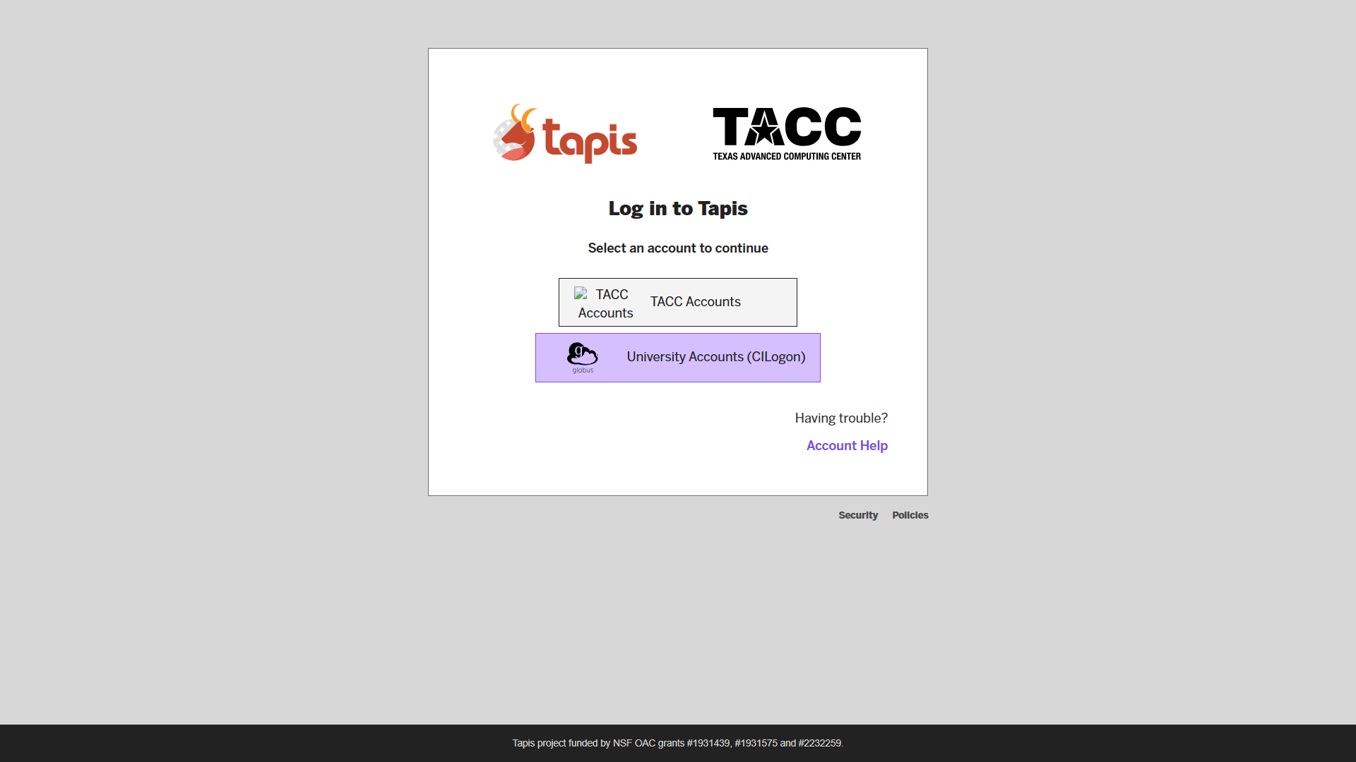
2. Select the University that you are affiliated with to log in.

3. After logging in you will be shown the main page for Icicle’s TAPIS.

4. To use this application, a system needs to be authenticated. We’ll use SDSC’s Expanse portal for this demonstration: https://portal.expanse.sdsc.edu/

   • You may log in using the ACCESS/CILogon account created beforehand.

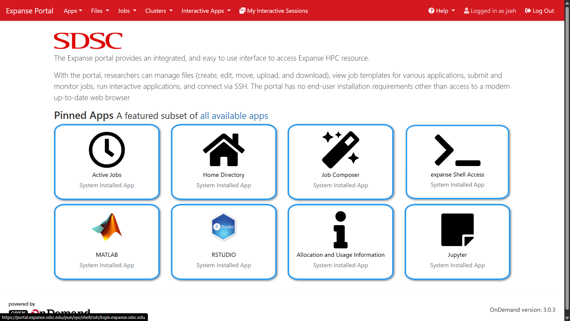
5. Once logged in, click on expanse Shell Access.

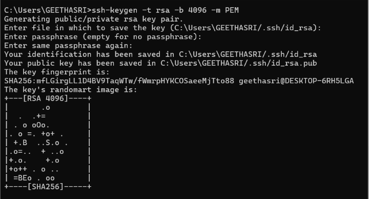
6. Inside the terminal, you will need to run these commands:

   ssh-keygen -t rsa -b 4096 -m PEM 
   cd ~/.ssh 
   cat id_rsa.pub
   cat id_rsa
   echo 'export SCRATCH="/expanse/scratch/${USER}"' >> ~/.bashrc
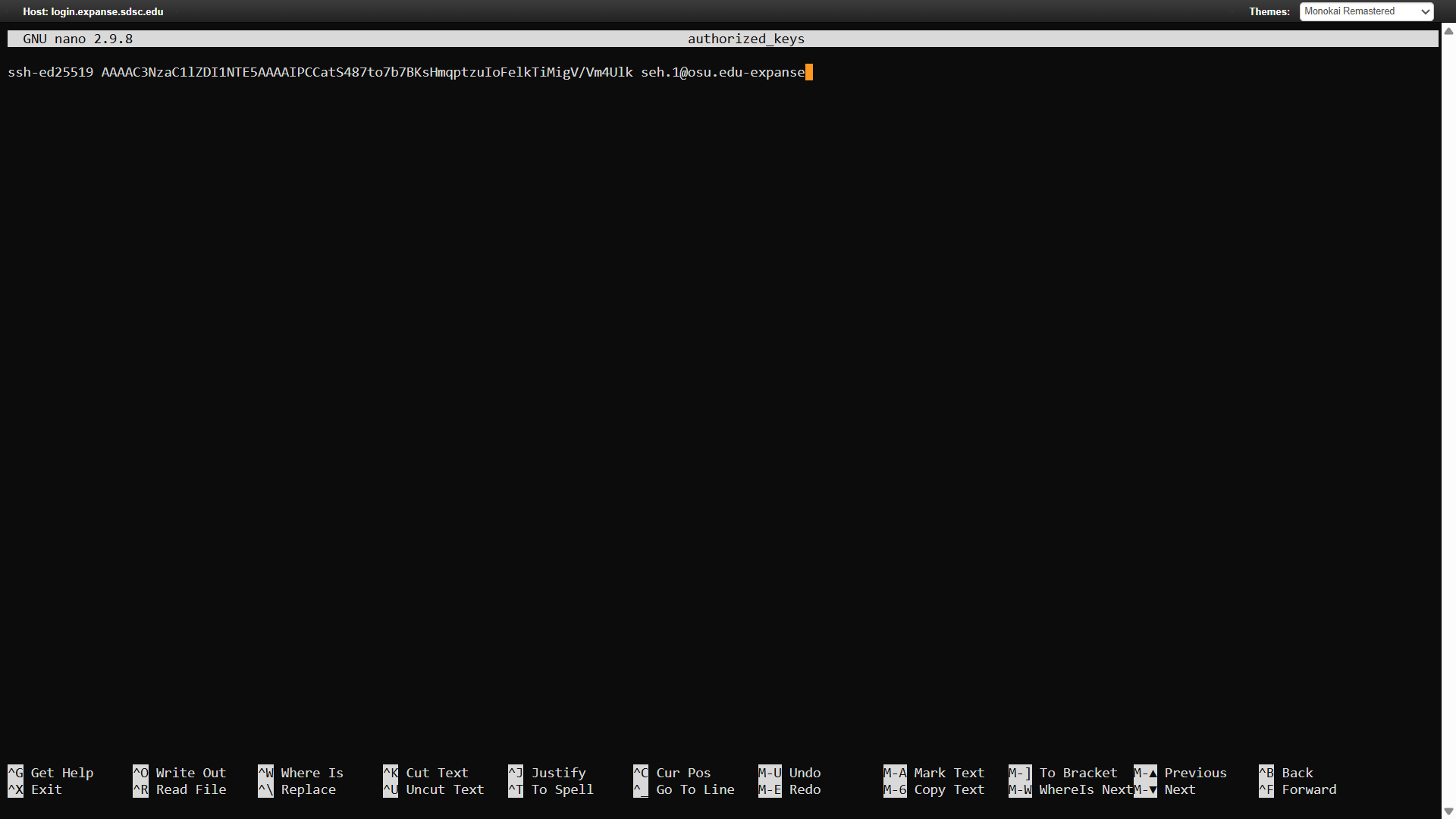
   echo 'export SCRATCH="/expanse/scratch/${USER}"' >> ~/.bash_profile

   id_rsa.pub is your public key and id_rsa is your private key. We will be using these to authenticate the Expanse system.

   In the terminal, run cd ~/.ssh and nano authorized_keys and paste the contents of your public key in. Run CTRL + X to save the contents of the file.

7. Log back into https://icicleai.tapis.io/ and click on Systems.

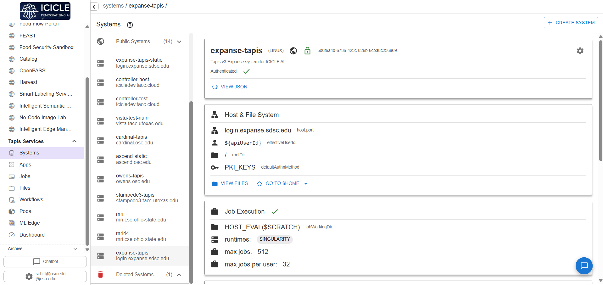
8. Click on the Authenticate button. The screen below will appear. Paste in your credentials generated from the keys made earlier into Private key and Public key and enter your username for that system in Login User.

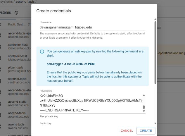
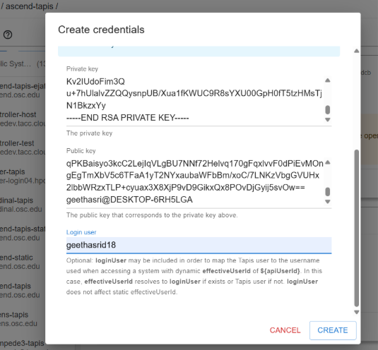
9. Your account should be authenticated now and should show this screen:

Common Issues

1. Double check that the entire public/private key is pasted into the box, including keys that may start with “----------- BEGIN RSA KEY —------------”. It's important to paste that in as well.
2. Ensure in authorized_keys your public key is pasted in and saved.
3. Ensure that the system you’re attempting to authenticate is the same system your authorized keys reside in.

---

Prerequisites

Please refer to the YAML Configuration Guide. This documentation is important as it goes over one of the key inputs for this application to run correctly.

Additionally, as noted in the YAML Configuration Guide, the application expects a specific dataset structure to run as expected. The program recursively takes each folder inside the directory as a label. For example:

    food/
         |_pasta/
             |_pizza/
            |_pepperoni_pizza/
             |_etc./

Pasta, pizza, pepperoni_pizza, and any other folder name will be taken as a label for the program. Images within its parent folder will be labeled as the parent folder’s name.

If you do not have a dataset, consider looking for one on Kaggle and please also refer to using KaggleHub for downloading the dataset into a directory.

Uploading to a System

This section demonstrates the steps to uploading the YAML configuration to a system.

1. Navigate to https://portal.expanse.sdsc.edu/
2. Under Files, click Home Directory.

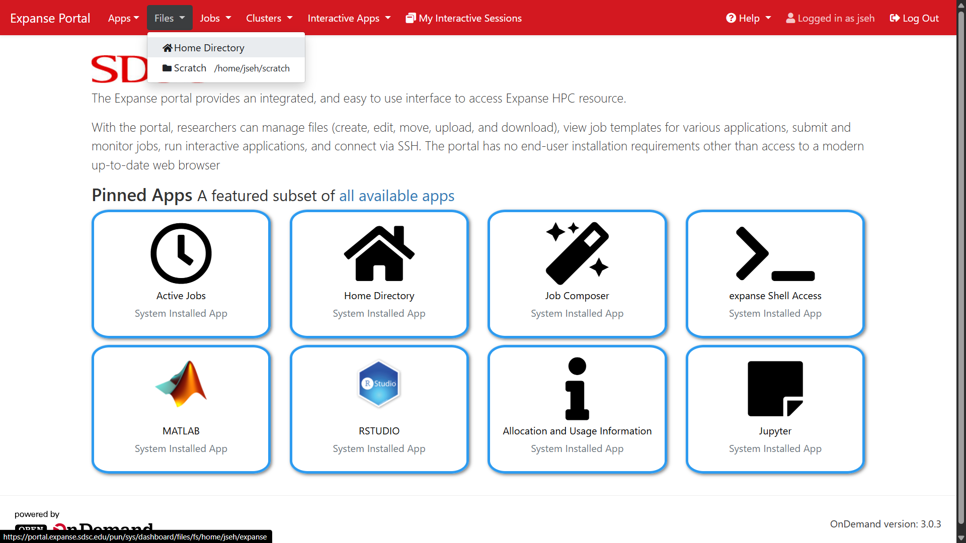
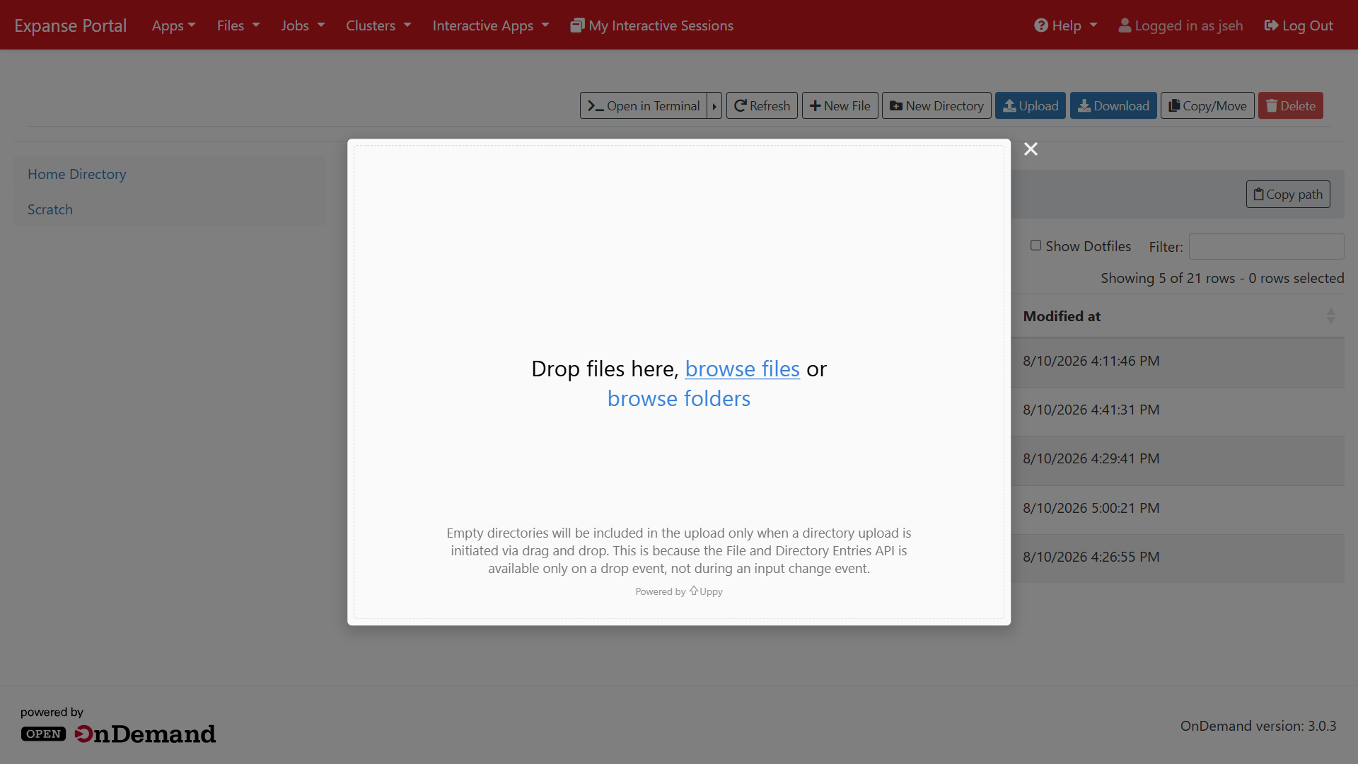
3. Click on Upload and here you may upload the configuration you created.

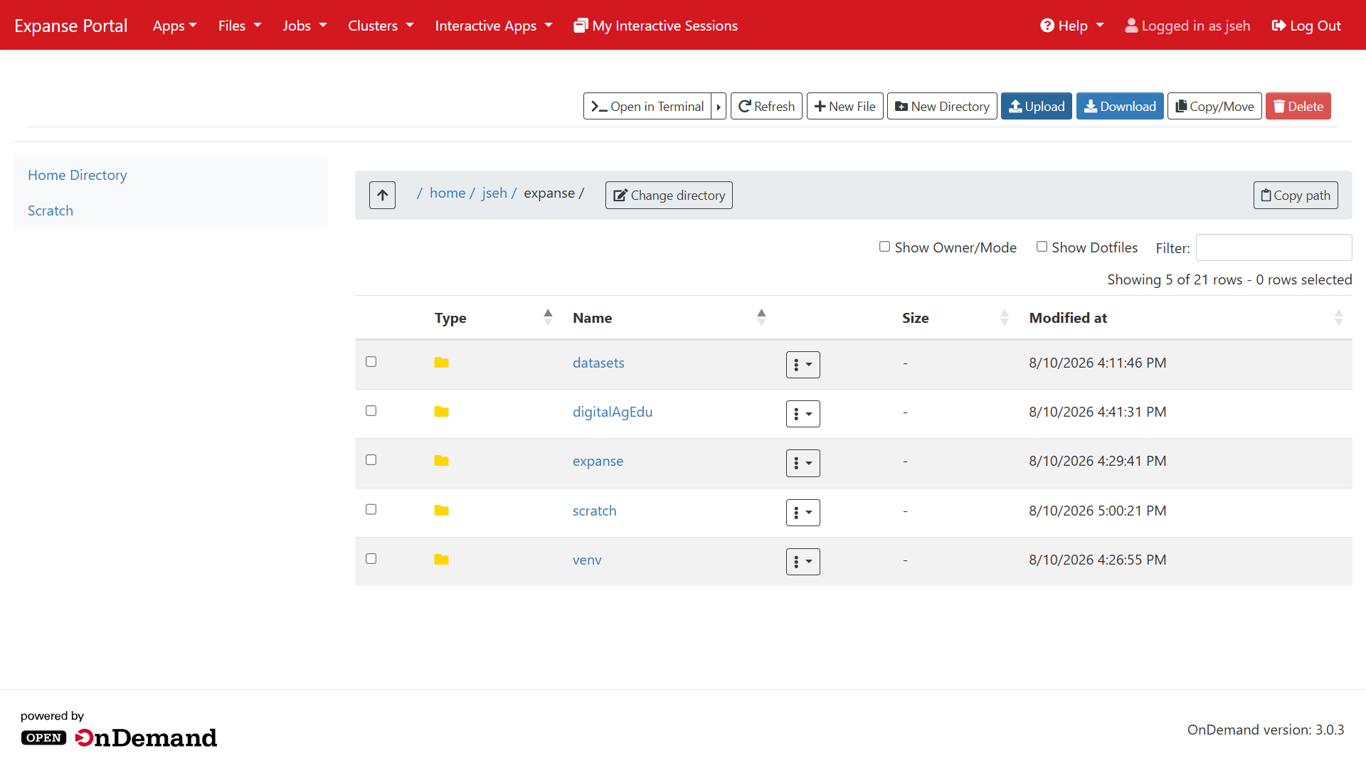
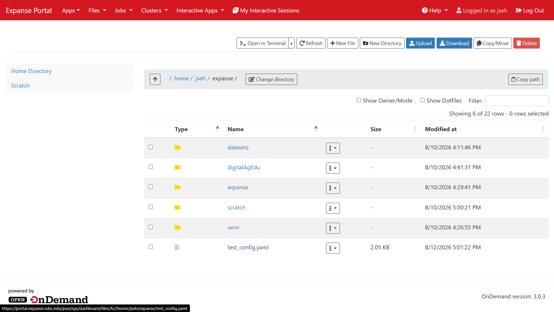
4. The path to your configuration file can be found by clicking the Copy Path button, pasting that output, and appending “/{your config name}”.
   • For example: /home/jseh/expanse/test_config.yaml
5. Remember/Write down this file path.

---

Running the Application

1. Navigate to https://icicleai.tapis.io/
   • Under Tapis Services click on Apps.
   • From the sidebar, scroll down and click on digital-age-edu.

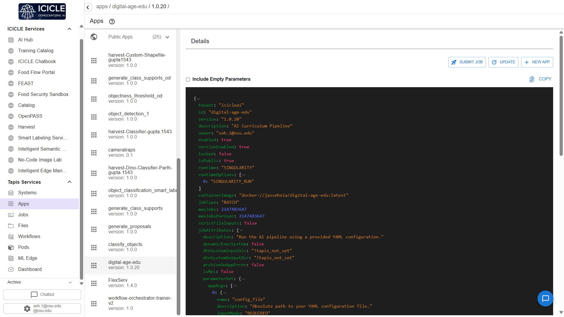
2. Click Submit Job. Afterwards click USE GUIDED JOB LAUNCHER.

3. This will pull up the Guided Job Launcher. This will be the main interface we use to start the application. Click Continue.

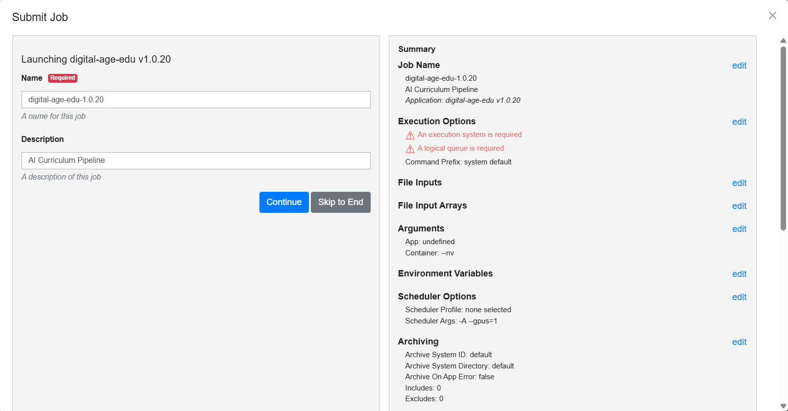
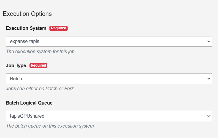
4. This is the Execution Options page. These determine the System the program will run on alongside the directory the program will run in.
   • Under Execution System select expanse-tapis-static (default).
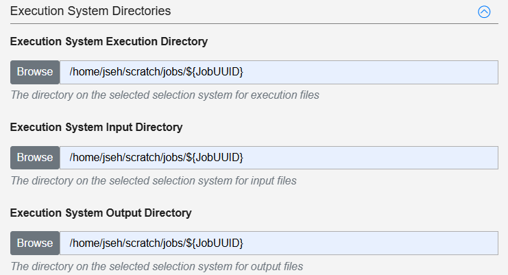
   • Under Batch Logical Queue select tapisGPUshared.
   • Under Execution System Execution Directory, Execution System Input Directory, and Execution System Output Directory, write down the path you want the application to run on. Append a “/${JobUUID}” to the end.
   • Remember/Write this down somewhere. Make sure it is a path on that system and a valid path on your account. For example: /home/<your_username>/${JobUUID}.

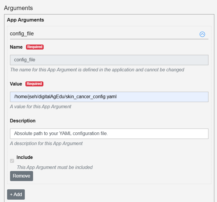
5. Click Continue until you reach Arguments. This section includes application arguments. We will be inputting the configuration created earlier. If you didn’t yet do so please refer back to Prerequisites.
   • Inside Value paste in the absolute path to the YAML configuration you created, for example mine would be: /home/jseh/expanse/test_config.yaml.

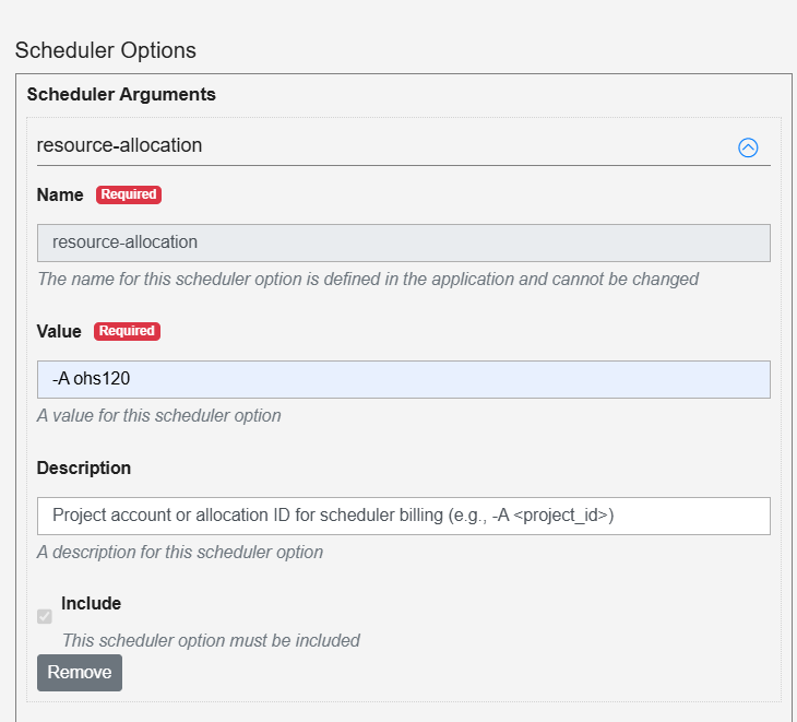
6. Click Continue until you reach Scheduler Options. In this section you define the id of your project to charge for usage.
   • By default, the community allocation -A uot260 is pre-filled so users do not need their own individual project account set up. If you have your own allocation, you may specify -A {Your Project ID} (found at https://portal.expanse.sdsc.edu/pun/sys/stats).

7. Click Continue until you reach the Job Submission page.
   • Click Submit Job.
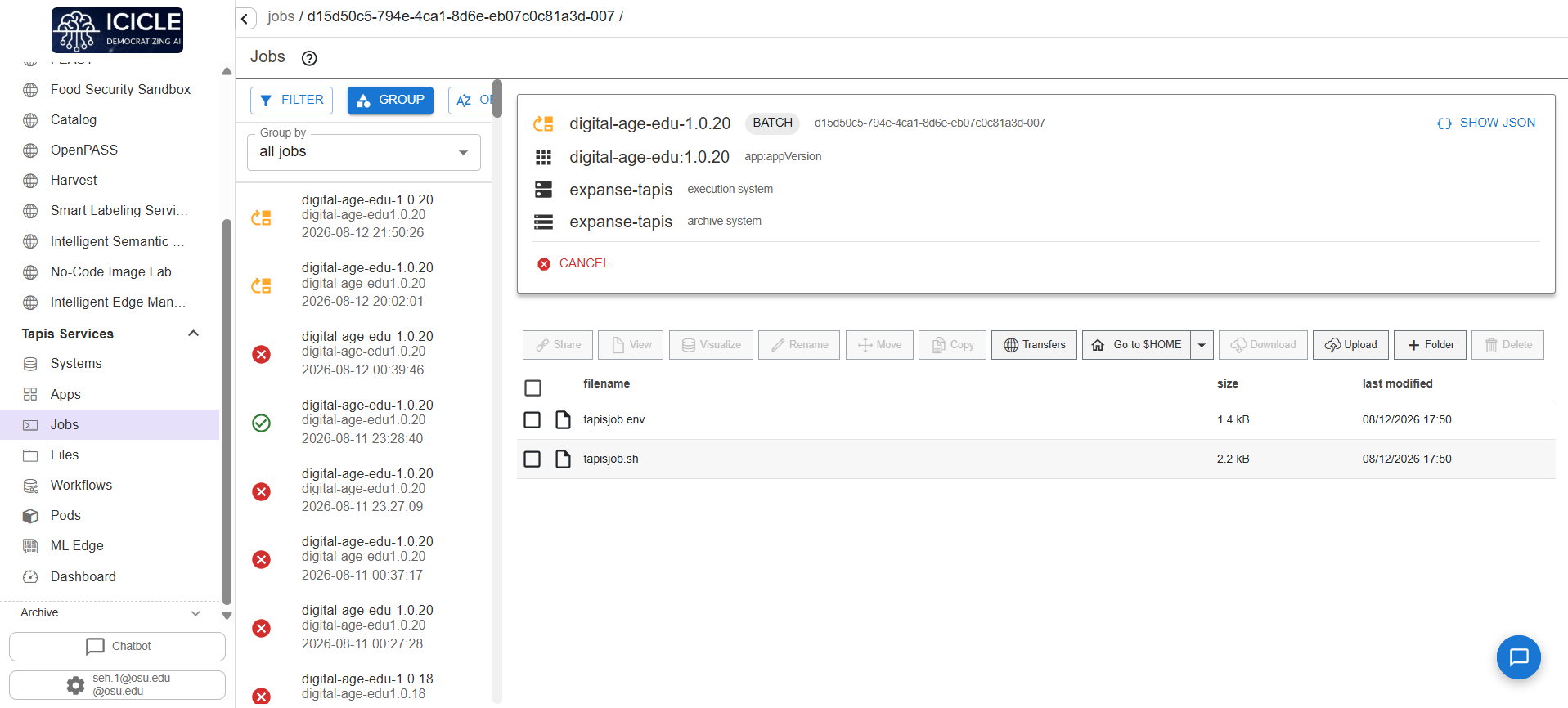
   • Keep note of the job id. In this example it is d15d50c5-794……..
   • Navigate back to the main page and click on Jobs.
   • Here you can see the job has been queued into Tapis. It will take some time for the application to run.
   • Please note to see any program text outputs it will be within tapisjob.out and you will need to reload the page to see current updates on the job status.

---

Understanding the Outputs

[!WARNING]

Critical Advisory: Download Results to Your Local Device

Expanse Static (expanse-tapis-static) is a community-managed execution system. File storage within shared and temporary scratch/job directories on Expanse Static is subject to periodic maintenance and may be wiped or cleared for storage management reasons.

Always download your generated outputs (curriculum markdown, exercises, reference solutions, metrics, plots, and models) to your local device or permanent institutional storage immediately after the job finishes.

The application is done running once in Jobs you see this:

Outputs

This section details the outputs of the program, how to use them, and overall expectations for after it runs.

1. models/

   • A .pth with weights to the trained DINOv2 model for classification
   • sam_vit_b_.pth weights for segmentation

2. {the output directory name defined in the config}/

   • results.json: Overall metrics for the pipeline and training/inference
   • class_mapping.json: Indexes the classes found to a number
   • confusion_matrix.png: Confusion matrix compiled from each fold
   • eval_confusion_matrix.png: Final model confusion matrix across entire dataset
   • curriculum.json: A json file for the curriculum
   • curriculum_{grade_level}.md: A markdown variant of the curriculum
   • cv_report.json: Model performance per fold
   • results.csv: The CSV containing metadata and data for every image

3. {the output directory name defined in the config}/exercises:

   • Week_{xx}/
     • Module/
       • concepts.md: markdown containing concepts needed for the given module
       • {concept}_exercise.py: The exercise for the student to complete. These are meant to be incomplete when generated so will fail when first ran
       • {concept}_solution.py: The solution to the exercise
       • {concept}_test.py: The test cases for the student to use
       • resources.md: Markdown containing resources for the module

4. {the output directory name defined in the config}/images

   • masks/: The mask used for segmentation
   • segmented/: The segmented image

---

Downloading Outputs to Your Local Machine

Because Expanse Static is community-managed and files may be purged over time, use the following methods to transfer the generated files to your personal computer:

1. Navigate to the Expanse Web Portal: https://portal.expanse.sdsc.edu/
2. In the top navigation bar, click Files -> Home Directory (or navigate to your scratch/execution directory).
3. Browse to your job's execution directory and enter the output folder.
4. Select the generated curriculum folder or archive and click Download in the upper action menu.

---

Accessing and Running Exercises on the System

This section goes over how to inspect and run the generated exercises directly on the cluster before or alongside downloading them.

1. Log into your system at https://portal.expanse.sdsc.edu/
2. Click on expanse Shell Access.
3. Inside the terminal execute the command:

   cd {the execution directory you saved, replacing ${JobUUID} with the job id}

   For example mine is:

   cd /home/jseh/scratch/jobs/5ce7ce30-50d0-47d1-91be-220c7e4ea26c-007

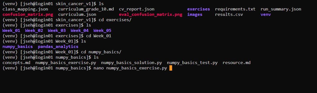
4. Execute ls. This will list the subdirectories within that directory.
5. Execute cd output. This changes your current directory into output.
6. Execute cd {what you named the directory}. Ex: my command is cd skin_cancer_v1.
7. Execute cd exercises. Here you will see the different modules.
8. For now we will go back to install the requirements. Run cd ../ to change directory into the parent folder.
   1. Run module load cpu/0.21.2a gcc/13.3.0/t46rsdv
   2. Run module load python/3.11.9/je56t6b
9. Run python -m venv venv. This will install the python virtual environment into the directory.
10. After it’s done installing run source venv/bin/activate.
11. Execute pip install uv.
12. Execute uv pip install -r requirements.txt. This will install all the requirement in parallel.
13. Execute cd exercises to get back into the exercises, run ls, and cd into a week.
14. You may run nano {the exercise name}_exercise.py to edit the contents of that week. Saving the contents, you can run python {the file name} to run the code within the file.

YAML Configuration Guide

Smart Curriculum Designer expects a YAML configuration to run correctly. This acts as the main point of freedom for educators to determine the content for their curriculum. Each parameter outlined here serves a purpose and unless otherwise specified needs to be filled out. Please refer to the sample YAML configuration listed below this document and on the line below. Additionally, please read the section Uploading to a System upon creating your config file.

A sample YAML configuration can be found here.

---

Implemented Parameters

Project

• domain: This is used by the VLM to define its background expertise.
• context_statement: A description of the problem. This is used by the automated curriculum generator to construct course topics, and by the VLM to structure its answers.
• use_case: Reserved for future extension. Changing this does not affect execution.

Dataset

• root_path: The absolute or relative path to the directory containing your images. Ensure the subfolders of the main directory are named the classes of the images. Eg:

  food/
       |_pasta/
       |_pizza/
       |_etc./

Output

• output: Configurations for the output
• directory: The destination folder where model predictions (results.csv), segmentation images, and execution logs will be written.

Pipeline

• stages: Sequential stages the pipeline will run. The stages run as such: Classification (DINOv2) -> Segmentation (SAM) -> VisualXAI (Grad-CAM)
• active: Toggles whether this stage runs. If set to false, the pipeline skips this model completely.
• prompt: Text inputs used for visual grounding:
  • For Segmentation: The text prompt describing the object to isolate (e.g., "the leaf", "the skin lesion").

Execution

• device: Set to "cuda" for fast GPU processing on machines with NVIDIA cards (or OSC cluster nodes). Set to "cpu" for slower, localized execution.
• batch_size: The number of images loaded into GPU memory at once. If you hit out-of-memory (OOM) errors, lower this value (e.g. from 16 to 4).
• image_size: Square resolution to resize input images. (518 is heavily recommended)
• max_samples: Set to a number (e.g. 20) to quickly test the pipeline on a small subset. Set to null to run over the entire dataset.
• seed: An integer locking randomness across Python, NumPy, and PyTorch, ensuring your cross-validation split and weight initialization remain 100% reproducible.

Curriculum

• subject & grade: Meta details printed on the generated lesson documents.
• weeks: Optional curriculum length. If omitted, the program will sum the weeks of the modules, or default to the amount of weeks for each module if modules.weeks is omitted too.
• modules:
  • id: The id of the module. Refer to the YAML sample for a full list of every module
  • week: The week the module will reside in. One week can have multiple modules.
• topics: Custom descriptions representing the core projects students will work on.
  • name: The name of the topic.
  • description: The description for the topic.
  • project: The project the topic is under.
• resources: Attaching resources relevant to the curriculum.
  • name: Name for the documentation.
  • url: URL leading to the documentation.

---

Uploading to a System

This section demonstrates the steps to uploading the YAML configuration to a system.

1. Navigate to https://portal.expanse.sdsc.edu/
2. Under Files, click Home Directory.

3. Click on Upload and here you may upload the configuration you created.

4. The path to your configuration file can be found by clicking the Copy Path button, pasting that output, and appending “/{your config name}”.
   • For example: /home/jseh/expanse/test_config.yaml
5. Remember/Write down this file path.

---

Sample YAML Config

# ==============================================================================
# BOILERPLATE CONFIGURATION FOR SMART CURRICULUM DESIGNER
# Instructions: Use this template for deploying new datasets on Tapis/OSC.
# Ensure all model_paths and dataset_roots point to PERSISTENT SHARED STORAGE
# ==============================================================================

# ===============
# Project Context
# ===============
project:
  domain: "<INSERT_DOMAIN> (e.g., Medical Imaging, Precision Agriculture)"
  context_statement: "<INSERT_CONTEXT> (e.g., diagnosing leaf diseases from images)"
  use_case: "educational_curriculum"

# ================
# Dataset Settings
# ================
dataset:
  # IMPORTANT NOTE: Point this to a persistent storage path
  root_path: "/path/to/shared/persistent/storage/dataset_folder"

output:
  # Output directory where results will be generated
  directory: "./outputs/experiment_v1"

# ================
# Pipeline Stages
# ================
pipeline:
  stages:
    - name: "Classification"
      active: true
      task_type: "<INSERT_TASK_TYPE>"

    - name: "Segmentation"
      active: true
      task_type: "object_extraction"
      prompt: "<INSERT_TARGET_OBJECT> (e.g., the skin lesion, the diseased leaf)"

    - name: "VisualXAI"
      active: false # Explainable AI / Attention Maps
      task_type: "visual_explainability"

# ============
# Execution
# ============
execution:
  device: "cuda" # Required for DINOv2 performance
  batch_size: 16
  image_size: 518
  max_samples: null # Set to an integer (e.g., 50), null for full dataset
  seed: 42

# ==================
# Curriculum Config
# ==================
curriculum:
  subject: "<INSERT_COURSE_SUBJECT>"
  grade: 10
  weeks: 24

  modules:
  # Explicit per-week assignments (multiple modules can share the same week)
    - id: "numpy_basics"
      week: 1
    - id: "pandas_analytics"
      week: 1
    - id: "pytorch_basics"
      week: 2
    - id: "interactive_segmentation"
      week: 3
    - id: "image_datasets"
      week: 4
    - id: "custom_cnn"
      week: 4
    - id: "cnn_optimization"
      week: 4
    - id: "transfer_learning"
      week: 4
    - id: "semantic_segmentation"
      week: 4
    - id: "explainable_ai"
      week: 5
    - id: "vector_embeddings"
      week: 5
    - id: "gradio_deployment"
      week: 6

  topics:
    - name: "<INSERT_TOPIC_NAME>"
      description: "<INSERT_TOPIC_DESCRIPTION>"
      project: "<INSERT_PROJECT_NAME>"

  resources:
    - name: "Dataset Source"
      url: "<INSERT_DATASET_URL>"

Curriculum Modules & Concepts Guide

This guide provides a comprehensive overview of the curriculum modules generated by Smart Curriculum Designer. It details the pedagogical goals, mathematical foundations, core programming exercises, and learning outcomes for each topic across the computer vision and machine learning curriculum.

Table of Contents

1. Module 1: NumPy Array Basics, Vectorization & Performance
2. Module 2: Pandas Data Wrangling & Matplotlib Visualizations
3. Module 3: PyTorch Foundations & Neural Network Lifecycle
4. Module 4: Interactive Image Segmentation with OpenCV
5. Module 5: Custom PyTorch Datasets, Transforms & DataLoaders
6. Module 6: Custom Convolutional Neural Networks (CNNs)
7. Module 7: CNN Optimization, Regularization & Checkpoints
8. Module 8: Transfer Learning & Backbone Benchmarking
9. Module 9: Semantic Segmentation & Dense U-Net Decoders
10. Module 10: Explainable AI & Grad-CAM Attributions
11. Module 11: Image Embeddings, PCA Clustering & Vector Search
12. Module 12: Capstone Integration & Gradio Deployment
13. Module 13: Vision-Language Models (VLM) & Multimodal VQA
14. Supplementary Student & Instructor Deliverables

Module 1: NumPy Array Basics, Vectorization & Performance

Pedagogical Goal

Establishes that in computer vision, images are 3D numerical matrices of shape $(H, W, C)$. Students master fast, hardware-accelerated matrix operations and learn to avoid slow Python for loops when handling high-resolution visual data.

Core Concepts & Mathematics

• Multidimensional Arrays (Ndarrays): Memory-contiguous pixel grids for fast CPU hardware retrieval.
• Z-Score Normalization: $$\mu = \frac{1}{N} \sum x_i, \quad \sigma = \sqrt{\frac{1}{N} \sum (x_i - \mu)^2}, \quad Z_i = \frac{x_i - \mu}{\sigma}$$ Standardizes input distributions to prevent early gradient scaling anomalies during neural network training.
• Broadcasting: Performing arithmetic operations on arrays of mismatched shapes without copying memory (e.g., subtracting a $(3,)$ channel mean vector from a $(224, 224, 3)$ image).
• SIMD Vectorization: Replacing interpreter loops with compiled C-level Single Instruction, Multiple Data operations.

Key Functions & Student Exercises

1. create_and_reshape_arrays(): Creates 1D numerical sequences and reshapes them into 2D matrices, zero arrays, and ones arrays.
2. slice_and_crop(mock_image): Extracts bounding regions of interest using coordinate slicing [y_start:y_end, x_start:x_end, :].
3. apply_broadcasting(image, mean_vector, mask): Normalizes pixel values to $[0.0, 1.0]$, centers by channel mean, and applies a 2D spatial binary mask.
4. elementwise_math(arr): Vectorized squaring, linear shifting, and bounds restriction using np.clip.
5. statistics_and_standardization(arr): Extracts global mean, standard deviation, min, max, and handles divide-by-zero variance cases.
6. boolean_thresholding(image, threshold): Creates boolean masks for pixel filtering.
7. matrix_multiplication(w, x): Transposition and matrix dot-product operations using the @ operator.
8. loop_vs_vectorization_benchmark(size): Performance benchmark measuring execution speedup of NumPy vectorization over pure Python loops.
9. Bonus Challenge — extract_patches(image, patch_size, stride): Slices large high-resolution images into uniform spatial tiles (essential for gigapixel pathology and satellite scans).

Module 2: Pandas Data Wrangling & Matplotlib Visualizations

Pedagogical Goal

Teaches students how to inspect model prediction logs (results.csv), extract error patterns, and conduct active learning error audits to identify model blind spots and prioritize dataset re-annotation.

Core Concepts & Mathematics

• Classification Accuracy Metric: $$\text{Accuracy} = \frac{TP + TN}{TP + TN + FP + FN}$$
• Error Mining & Active Learning: Sorting prediction logs by confidence to isolate high-confidence incorrect predictions ("hard negatives") for targeted data re-collection.
• Data Hygiene: Handling missing values (NaNs) safely without introducing statistical data leakage between training and validation distributions.

Key Functions & Student Exercises

1. explore_and_inspect_data(csv_path): Loads tabular CSV logs, inspecting structure via .head(), .tail(), .info(), and .describe().
2. select_and_filter_data(df): Slices columns and isolates misclassified samples where predicted_class != ground_truth.
3. feature_engineering(df): Creates boolean flags is_correct and categorical error descriptions error_type.
4. sort_and_find_extremes(df): Sorts samples to identify extreme failure modes.
5. group_statistics(df): Performs groupby("ground_truth") aggregations to measure per-class sample counts and precision rates.
6. handle_missing_values(df): Cleans corrupted logs via .fillna() and .dropna().
7. create_matplotlib_visualizations(df, plot_dir): Generates multi-panel figures:
   • Training vs. validation loss curve comparisons.
   • Per-class classification accuracy bar charts.
   • Misclassification distribution histograms.
   • Overall correctness pie charts.
8. Bonus Challenge — find_hardest_samples(df, class_name, top_n): Mines the top $K$ worst mistakes for a specific class to prioritize dataset re-annotation.

Module 3: PyTorch Foundations & Neural Network Lifecycle

Pedagogical Goal

Demystifies neural network internals. Students build a Multi-Layer Perceptron (MLP) from scratch in PyTorch, trace Autograd gradient graphs, and write the complete training and validation lifecycle.

Core Concepts & Mathematics

• Binary & Multi-Class Cross-Entropy Loss: $$L_{BCE} = -\frac{1}{N} \sum_{i=1}^N \left[ y_i \log(p_i) + (1 - y_i) \log(1 - p_i) \right]$$
• Softmax Probability Mapping: $$P(y = c \mid z) = \frac{e^{z_c}}{\sum_{j=1}^C e^{z_j}}$$
• Autograd & The Training Lifecycle Step:
  1. optimizer.zero_grad() $\to$ Reset accumulated gradients.
  2. outputs = model(inputs) $\to$ Forward pass.
  3. loss = criterion(outputs, targets) $\to$ Compute objective penalty.
  4. loss.backward() $\to$ Compute exact parameter gradients via the chain rule.
  5. optimizer.step() $\to$ Update weights using gradient descent.

Key Functions & Student Exercises

1. tensor_basics(python_list): Converts Python lists to float tensors, generates normal distributions, and handles GPU (cuda) device mapping.
2. compute_autograd_gradient(x_value): Defines scalar functions on leaf tensors with requires_grad=True and computes analytic derivatives.
3. SimpleImageMLP: Inherits from nn.Module, defining nn.Linear layers, nn.ReLU activations, and flattening $(B, C, H, W)$ tensors to $(B, C \cdot H \cdot W)$.
4. inspect_forward_shapes(model, x): Traces spatial dimension contraction through intermediate layers.
5. count_trainable_parameters(model): Calculates total parameters where p.requires_grad == True.
6. logits_to_probabilities(logits): Converts unbounded decision logits into probability vectors using torch.softmax and torch.argmax.
7. train_step() & validation_step(): Implements isolated training and validation execution modes (model.train() vs model.eval() with torch.no_grad()).
8. calculate_accuracy_manually() & calculate_confusion_matrix_manually(): Builds $C \times C$ confusion matrices directly using tensor comparison logic.
9. train_model(): Complete multi-epoch training orchestrator featuring index shuffling, batch iterations, validation tracking, and .pth weight saving.
10. Bonus Challenge — train_step_with_l2(model, ..., l2_lambda): Manually calculates and injects an L2 weight decay penalty ($\frac{\lambda}{2}\sum w^2$) into the loss before backpropagation.

Module 4: Interactive Image Segmentation with OpenCV

Pedagogical Goal

Contrasts classical computer vision heuristics (seed-based FloodFill) with deep learning foundation models (Segment Anything / SAM), providing an interactive GUI to explore pixel connectivity.

Core Concepts & Mathematics

• Spatial Image Moments & Centroids: $$M_{ij} = \sum_{x,y} x^i y^j I(x,y), \quad cX = \frac{M_{10}}{M_{00}}, \quad cY = \frac{M_{01}}{M_{00}}$$
• Intersection over Union (IoU / Jaccard Index): $$\text{IoU}(A, B) = \frac{|A \cap B|}{|A \cup B|}$$
• Breadth-First Search (BFS) FloodFill: Propagating mask boundaries based on color differences (loDiff/upDiff) vs. deep semantic feature attention in SAM.

Key Functions & Student Exercises

1. inspect_image(image): Retrieves height, width, dtype, and color channels.
2. convert_color_spaces(image): Converts BGR arrays into display RGB, luminance Grayscale, and color-filtering HSV.
3. threshold_image(image, threshold_value): Applies binary intensity thresholding.
4. floodfill_segmentation(image, seed_point, tolerance): Applies seed-point FloodFill with border padding.
5. calculate_iou(mask_a, mask_b): Computes spatial overlap similarity between classical masks and pipeline SAM masks.
6. create_overlay(image, mask, color, alpha): Blends color masks onto images via cv2.addWeighted.
7. find_and_draw_contours() & get_bounding_box(): Computes outer contour vectors and minimum bounding rectangles $(x, y, w, h)$.
8. Interactive GUI / Headless Fallback: Real-time OpenCV window listening to mouse clicks, tolerance adjustment keys (+/-), and generating side-by-side comparison overlays against SAM.
9. Bonus Challenge — calculate_mask_centroid(mask): Uses spatial moments (cv2.moments) to locate the center-of-mass coordinates of segmented regions.

Module 5: Custom PyTorch Datasets, Transforms & DataLoaders

Pedagogical Goal

Teaches scalable, memory-efficient data engineering for computer vision on supercomputers. Students implement custom Dataset classes using on-the-fly lazy loading to avoid RAM exhaustion.

Core Concepts & Mathematics

• Dataset-Wide Channel Normalization: $$\mu_c = \frac{1}{N \cdot H \cdot W} \sum_{i=1}^N \sum_{y=1}^H \sum_{x=1}^W I_c(i, y, x)$$
• Pipeline Shape Transitions: $$\text{PIL Image }(H, W, C) \xrightarrow{\text{ToTensor}} \text{Tensor }(C, H, W) \xrightarrow{\text{DataLoader}} \text{Batch }(B, C, H, W)$$
• Data Augmentation: Preserving semantic labels while introducing geometric perturbations (random flips, rotations) on training sets, while keeping validation sets strictly deterministic.

Key Functions & Student Exercises

1. split_dataset(image_paths, train_ratio, seed): Generates reproducible train/test splits.
2. CustomImageDataset: Inherits from torch.utils.data.Dataset, implementing:
   • __len__: Returns total valid image file paths (filtering OS artifacts like .DS_Store).
   • __getitem__: Dynamically opens images via PIL, extracts directory class labels, applies transforms, and returns (tensor, label).
3. build_transforms() & build_augmentation_transforms(): Constructs transforms.Compose pipelines with resizing, horizontal flips, rotations, tensor casting, and ImageNet standardization.
4. inspect_transform_flow(): Traces structural dimension changes at each preprocessing step.
5. calculate_dataset_statistics(): Scans directory hierarchies to identify class distribution imbalances.
6. validate_batch(): Sanity-checks batches for NaNs, 4D shape validity, float32 dtypes, and label index ranges.
7. visualize_batch(): Un-normalizes tensors and plots $4 \times 4$ image grids with class titles.
8. compare_shuffle_effect(): Demonstrates how shuffle=True breaks class ordering biases across training epochs.
9. Bonus Challenge — calculate_dataset_stats(dataset, max_samples): Computes dataset-specific channel mean and standard deviation vectors across all images.

Module 6: Custom Convolutional Neural Networks (CNNs)

Pedagogical Goal

Transitions students from MLPs to Convolutional Neural Networks. Explains how sliding kernel filters preserve spatial locality and reduce parameters through weight sharing.

Core Concepts & Mathematics

• Convolutional Output Dimension Arithmetic: $$O = \left\lfloor \frac{I - K + 2P}{S} \right\rfloor + 1$$
• Learnable Parameter Count for Conv Layers: $$\text{Params} = C_{out} \cdot (C_{in} \cdot K^2 + 1)$$
• Receptive Field Expansion: How stacking small $3 \times 3$ filters and pooling layers expands the effective visual area captured by deeper neurons.

Key Functions & Student Exercises

1. CustomCNN: Constructs a 2-stage CNN architecture containing nn.Conv2d(3 $\to$ 8), nn.MaxPool2d(2, 2), nn.Conv2d(8 $\to$ 16), nn.MaxPool2d(2, 2), and a linear classification head.
2. count_parameters(model): Calculates total learnable parameters.
3. trace_cnn_shapes(model, sample_tensor): Records tensor dimension changes through convolution, activation, pooling, and flattening layers.
4. extract_first_layer_activations(): Intercepts and extracts early feature map activations.
5. visualize_pooling_effect(): Plots feature maps before and after max-pooling side-by-side to visualize spatial compression.
6. visualize_feature_maps(): Renders a $2 \times 4$ grid showing the input image alongside its first 7 convolutional filter responses (initialized with Sobel and Laplacian edge filters).
7. softmax_predictions(): Maps raw network logits to percentage probabilities.
8. Bonus Challenge — cnn_block_analysis(input_height, input_width): Calculates final output activation shapes, combined parameter counts, and raw memory footprint in bytes.

Module 7: CNN Optimization, Regularization & Checkpoints

Pedagogical Goal

Teaches techniques for stabilizing model training on supercomputers, combating overfitting, and creating resilient validation checkpoint pipelines.

Core Concepts & Mathematics

• Step Learning Rate Decay: $$\eta_t = \eta_0 \cdot \gamma^{\lfloor t / s \rfloor}$$
• Batch Normalization (BatchNorm2d): Standardizing batch activations to accelerate convergence and reduce sensitivity to initialization.
• Dropout Regularization: Randomly zeroing neuron activations during training to force redundant feature representations.

Key Functions & Student Exercises

1. RegularizedCNN: Implements a CNN with toggles for BatchNorm2d and Dropout across stages.
2. optimize_model_hyperparameters(): Configures an Adam optimizer with L2 weight decay and a StepLR scheduler.
3. validation_checkpoint_step(): Monitors validation loss, serializing .pth state dictionaries when performance reaches a new minimum.
4. compare_baseline_vs_optimized(): Runs side-by-side training comparing unregularized baseline models against regularized networks over 15 epochs.
5. plot_weight_distributions(): Plots histograms of convolutional weights to show how regularization prevents extreme weight spikes.
6. simulate_checkpointing_story(): Terminal simulation demonstrating how checkpoints restore the best model state after overfitting occurs.
7. Bonus Challenge — audit_checkpoint_integrity(model, checkpoint_path, ...): Audits saved .pth checkpoint files for shape mismatches, key completeness, and optimizer/scheduler state consistency before loading.

Module 8: Transfer Learning & Backbone Benchmarking

Pedagogical Goal

Explains why foundation vision models achieve high accuracy on small datasets. Students configure layer freezing, fine-tune ResNet architectures, and benchmark predictions against DINOv2 pipeline outputs.

Core Concepts & Mathematics

• Hierarchical Visual Primitives: Early layers detect universal edges and shapes; late layers detect domain-specific semantics.
• Cosine Proximity in Feature Space: $$\text{Cosine}(A, B) = \frac{A \cdot B}{|A| \cdot |B|}$$
• Freezing vs. Discriminative Fine-Tuning: Locking early feature extractors (requires_grad = False) vs. unfreezing high-level residual blocks (layer4).

Key Functions & Student Exercises

1. get_resnet_model(num_classes, mode): Configures ResNet18 in "frozen" (head only) or "unfrozen_last_block" modes.
2. count_trainable_parameters(): Compares trainable parameter counts (thousands vs. millions).
3. visualize_feature_reuse(): Compares activations from randomly initialized filters against structured, pretrained ResNet filters on the same image.
4. run_10_image_comparison(): Evaluates a 10-image slice, generating an audit table comparing DINOv2 vs. ResNet predictions and confidence scores.
5. Bonus Challenge — classify_with_prototypes(query_embedding, class_prototypes): Implements a nearest class prototype classifier using Cosine Similarity for few-shot learning.

Module 9: Semantic Segmentation & Dense U-Net Decoders

Pedagogical Goal

Bridges classification and dense pixel-wise prediction. Students build a transposed-convolution decoder to rebuild spatial resolution from compressed bottleneck features.

Core Concepts & Mathematics

• Soft Dice Loss Optimization: $$L_{Dice} = 1 - \frac{2 \sum (p_i \cdot g_i) + \epsilon}{\sum p_i^2 + \sum g_i^2 + \epsilon}$$
• Combined Segmentation Loss: $$L_{\text{Total}} = L_{\text{BCEWithLogits}} + L_{\text{Dice}}$$
• Learned Upsampling & Skip Connections: Using ConvTranspose2d to expand spatial dimensions while highlighting why skip connections are necessary to recover fine border contours.

Key Functions & Student Exercises

1. MiniSegmentationDecoder: Implements a multi-stage upsampler using nn.ConvTranspose2d (kernel=4, stride=2, padding=1) with dimension validation assertions.
2. compute_hard_dice(): Calculates the non-differentiable Dice Similarity Coefficient (DSC) on boolean thresholded masks.
3. compute_soft_dice(): Computes the differentiable Soft Dice coefficient across spatial dimensions.
4. combined_loss(): Implements a composite loss function combining BCE with logits and Soft Dice loss.
5. find_optimal_threshold(): Searches candidate thresholds $[0.1, 0.9]$ to maximize the Jaccard/Dice overlap score against ground-truth SAM masks.

Module 10: Explainable AI & Grad-CAM Attributions

Pedagogical Goal

Teaches model transparency and auditability. Students use PyTorch hooks to capture gradients and feature maps, projecting visual heatmaps that show why a model made a specific prediction.

Core Concepts & Mathematics

• Grad-CAM Attribution Weighting: $$\alpha_c^k = \frac{1}{Z} \sum_{i,j} \frac{\partial Y^c}{\partial A_{i,j}^k}, \quad L_{\text{Grad-CAM}}^c = \text{ReLU}\left( \sum_k \alpha_c^k A^k \right)$$
• Attribution vs. Segmentation: Segmentation identifies what is present; attribution identifies what influenced the decision.
• Class Sensitivity & Cautions: Verifying that heatmaps change when switching target classes, and understanding failure modes (gradient saturation, spurious correlations).

Key Functions & Student Exercises

1. GradCAMHook: A Python context manager that registers and removes PyTorch forward and backward hooks on target convolutional layers.
2. generate_gradcam(): Computes channel gradient weights, computes the weighted sum of feature maps, applies ReLU, and normalizes the heatmap to $[0.0, 1.0]$.
3. generate_saliency_map(): Computes vanilla pixel-wise input gradients ($\max_c |\nabla_X Y^c|$).
4. test_class_switch_stability(): Evaluates class sensitivity by generating heatmaps for Class A vs. Class B on the same image and computing their overlap IoU.
5. Bonus Challenge — postprocess_heatmap(cam, threshold): Implements a $3 \times 3$ box-blur smoothing filter and threshold binarizer to clean attribution overlays.
6. Bonus Challenge — compute_heatmap_overlap(heatmap1, heatmap2): Computes quantitative IoU overlap between two distinct heatmaps.

Module 11: Image Embeddings, PCA Clustering & Vector Search

Pedagogical Goal

Connects spatial feature maps to high-dimensional latent embeddings. Students implement vector similarity search and dimensionality reduction for clustering analysis.

Core Concepts & Mathematics

• Cosine Similarity (Angular Alignment): $$\text{Cosine}(A, B) = \frac{A \cdot B}{|A| \cdot |B|}$$
• Magnitude Invariance: Why Cosine Similarity ignores vector length (intensity/brightness) to focus purely on semantic direction.
• PCA Dimensionality Reduction: Projecting high-dimensional representations to 2D for visual inspection while querying full-dimensional vectors in production search.

Key Functions & Student Exercises

1. compute_cosine_similarity(vec_a, vec_b): Computes angular alignment between 1D representation vectors.
2. project_to_2d(embeddings, n_components=2): Uses Principal Component Analysis (PCA) to compress high-dimensional vectors to 2D coordinates.
3. semantic_search(query_embedding, database_embeddings, top_k): Performs cosine nearest-neighbor search across an image vector database.
4. plot_embedding_clusters(): Renders color-coded 2D scatter plots of projected image clusters.
5. Bonus Challenge — compute_euclidean_distance(vec_a, vec_b): Computes magnitude-sensitive Euclidean distance ($\sqrt{\sum (A_i - B_i)^2}$) to compare against Cosine metric behaviors.

Module 12: Capstone Integration & Gradio Deployment (Work In Progress)

Pedagogical Goal

The capstone integration module. Students combine their trained classification model, segmentation overlays, and explainability heatmaps into a full-stack interactive web application using Gradio.

Core Concepts & Workflows

• End-to-End Inference Pipelines: Wrapping preprocessing, forward prediction, FloodFill/SAM segmentation, and saliency map extraction into a unified execution handler.
• Client-Server ML Architectures: Exposing model capabilities through responsive UI components (image uploaders, confidence sliders, image overlays).
• Input Sanitation: Auditing user-uploaded images for corruption or flat variance before executing GPU passes.

Key Functions & Student Exercises

1. load_model_weights(model_path, num_classes): Instantiates models and safely loads serialized .pth state dictionaries with fallback handling.
2. segment_image_fallback(): Generates transparent green segmentation overlays.
3. generate_saliency_map(): Generates pixel-wise attribution overlays for web rendering.
4. run_pipeline(model, image_numpy, classes): Unified inference pipeline returning (predicted_class, confidence, segmentation_overlay, saliency_map).
5. Gradio Web Interface Launch: Constructs gr.Interface with image upload inputs, prediction textboxes, confidence sliders, and dual visual diagnostic display panels.
6. Bonus Challenge — get_image_pixel_statistics(image_numpy): Computes uploaded image pixel statistics (mean, std, min, max) to validate input quality.

Supplementary Student & Instructor Deliverables

Alongside the coding exercises, each module automatically generates supporting documentation:

1. concepts.md (Module Theoretical Guide)

Generated inside each weekly exercise folder to serve as an on-demand textbook chapter:

• Core Concepts: Detailed explanations of visual representations, layer architectures, and engineering principles.
• Mathematical Formulations: LaTeX equations, complete variable definitions, and machine learning rationale.
• Key Functions & Real-World Relations: Algorithmic workflows and industry applications.
• Practical Failure Cases & Pitfalls: Common software bugs (e.g., coordinate axis swapping in OpenCV, forgetting optimizer.zero_grad(), SettingWithCopyWarning in Pandas).

2. resource.md (Curated References & Reading Lists)

Generated inside each weekly exercise folder with curated external links:

• Official Documentation: Direct links to PyTorch, NumPy, Pandas, OpenCV, and Gradio guides.
• Visual & Interactive Explanations: 3Blue1Brown animations, CNN Explainer 3D tools, Distill.pub articles, and Stanford CS231n notes.
• Bonus Challenge Prompts: Guidance on optional extension exercises.

3. curriculum_[grade_level].md (Course Syllabus)

Generated in the root output directory to outline the full course schedule:

• Empirical Pipeline Run Metrics: Total images processed, baseline accuracy achieved, and GPU execution time per stage.
• Classroom Case Studies: Direct file paths to sample images that the model classified correctly (true positives) and incorrectly (false positives/negatives) for classroom discussion.
• Dataset Summary: Number of classes, imbalance ratio, size category, and suggested evaluation metrics.
• Weekly Schedule: Complete week-by-week calendar mapping each topic to hands-on coding labs.